Key questions we must address

Let’s address the same questions we did in the case of a pure Newton’s method for scalar functions.

• How do we recursively update \(x\) to approach \(x^*\)?
  • Answer: Standard descent methods use the following update term, \(x^{(k+1)}=x^{(k)}+t^{(k)}\Delta x^{(k)}\). While there is some freedom in our choice of \(t\) and \(\Delta x\), we must make sure that basic convex requirements hold; such as \(f(x^{(k+1)})<f(x^{(k)})\). What this means is that with each step we must be approaching a value of \(x\) that brings us closer to \(p^*\).
• How do we determine \(\Delta x_{nt}\)?
  • Answer: In the case of Newton’s method \(\Delta x_{nt}=-(\nabla^2f)^{-1}{\nabla f}\).
• How do we determine \(t\)?
  • Answer: We’ll use back-tracking to solve for each \(t^{(k)}\).

Deriving the Gradient and Hessian

Here we’ll show an example of a function and how to calculate both the gradient and hessian without using a package. The terms we derive will be used within our code later. Let’s consider

\[f(x)=-\sum_{i=1}^m \mathrm{log}(1-a_i^Tx)-\sum_{i=1}^n \mathrm{log}(1-x_i^2)\]

here \(x\in \mathbb{R}^n\), \(a\in \mathbb{R}^n\), but \(A\in \mathbb{R}^{m\times n}\). It is important to see that \(x_i\) is an element of the vector \(x\). Now we need to calculate the gradient, \(\nabla f(x)=\Big[ \frac{\partial f(x)}{\partial x_1},...,\frac{\partial f(x)}{\partial x_n}\Big]\). This works out to be

\[ \frac{\partial f(x)}{\partial x_j} =\frac{2x_j}{(1-x_j^2)}+\sum_{i=1}^m \frac{a_{ij}}{1-a_i^Tx} \] Lastly, we need to calculate the hessian, \(\nabla^2 f(x)=\Big[\big[\frac{\partial^2 f(x)}{\partial x_1^2},...\big],...\Big]\),

\[ \frac{\partial}{\partial x_k}\frac{\partial f(x)}{\partial x_j} = \delta_{jk}\Bigg( \frac{4x_j^2}{(1-x_j^2)^2} + \frac{2}{(1-x_j^2)} \Bigg) - \sum_{i=1}^m \frac{a_{ij}a_{ik}}{(1-a_i^Tx)^2} \]

Note that the partial derivative expression corresponds to an element of the Hessian matrix where k and j correspond to matrix row index and column index respectively.

Psuedo code for Newton’s Method

Now that we’ve calculated the important terms we can use Newton’s method to try and optimize our chosen function. To do this we will follow the procedure,

• Given:
  • \(x_0\), \(x \in \mathrm{dom}(f)\)
• Repeat:
  1. Compute \(\Delta x_{nt}\)
  2. Determine \(t\)
  3. Update \(x\)

Code for Newton’s Method

Now it’s time to code this thing up. Although I’m using python I will be trying to use basic structures that can be universally coded using any language. For those of you unfamiliar with the \([ \ ]\) list structure, this is similar to the \(\mathrm{Table}[ \ ]\) structure in mathematica.

To initialize our algorithm we will choose \(x_0\) to be a vector of zeros and \(A\) to be a matrix of random values.

#--------------------------------
#   Libraries
#--------------------------------
import sys
import numpy as np
from numpy.linalg import inv
import math
import random
import matplotlib.pyplot as plt

#--------------------------------
#   Modules
#--------------------------------

def f(A,x):
  # Return a scalar for a Matrix and vector input
  s1 = -sum([math.log(1-np.dot(a,x)) for a in A])
  s2 = -sum([math.log(1-xi**2) for xi in x])
  return s1+s2

def grad_f(A,x):
  #---  grad_f(A,x) = \nabla_x f(x)
  # Return a vector for a Matrix and vector input
  vec = [sum([a[j]/(1-np.dot(a,x)) for a in A])+2*xj/(1-xj**2) for j,xj in enumerate(x)]
  return np.asarray(vec) 

def hess_f(A,x,m,n):
  #---  hess_f(A,x) = \nabla_x^2 f(x)
  # Return a Matrix for a Matrix and vector input
  def dd(a,b):
    if a==b:
      return 1
    else:
      return 0
  mat = [[dd(j,k)*((4*xj**2)/(1-xj**2)**2+2/(1-xj**2))-sum([A[i][j]*A[i][k]/(1-np.dot(A[i],x))**2 for i in range(0,m)]) for j,xj in enumerate(x)] for k in range(0,n)]
  return np.asarray(mat)
  
#print f(A,x_in)
#print grad_f(A,x_in)
#print hess_f(A,x_in,m,n)

class Log:
  k=[]
  x=[]
  f=[]
  t=[]
  def __init__(self,name):
    self.name = name
  def record(self,k,x,f,t):
    self.k.append(k)  
    self.x.append(x)
    self.f.append(f)
    self.t.append(t)

def newtons_method(A,x0,m,n,kmax,alpha,beta,eta):
  #print 'Running newton_method() ...'
  log=Log('newtons_method')
  log.record(0,x0,f(A,x0),0)
  k=1 #initialize step number
  x=x0 #initialize x
  while k<kmax:
    grad = grad_f(A,x)
    hess = hess_f(A,x,m,n)
    inv_hess = inv(hess)
    x_step = -np.dot(inv_hess,grad)
    #Linesearch:backtracking from t=1
    t=1.
    while max(np.dot(A,np.add(x,t*x_step))) >= 1 or max(abs(np.add(x,t*x_step))) >=1:
      t=beta*t
    while f(A,np.add(x,t*x_step))<f(A,x)+alpha*t*np.dot(grad,x_step):
      t=beta*t
    x += t*x_step
    log.record(k,x,f(A,x),t)
    k+=1
  return log

#--------------------------------
#   Main
#--------------------------------

if __name__ == "__main__":

    #---------------------------------
    #   Run Solver
    #---------------------------------
    kmax=50
    beta=0.5
    alpha=0.01
    eta=0.1
    m=30
    n=30
    x0 = np.asarray([0. for i in range(0,n)])
    A = np.asarray([[random.uniform(0,1) for i in range(0,n)] for j in range(0,m)])
    log = newtons_method(A,x0,m,n,kmax,alpha,beta,eta)
    plt.plot(log.k,log.t)
    plt.title('t vs k')
    plt.show()
    plt.clf()
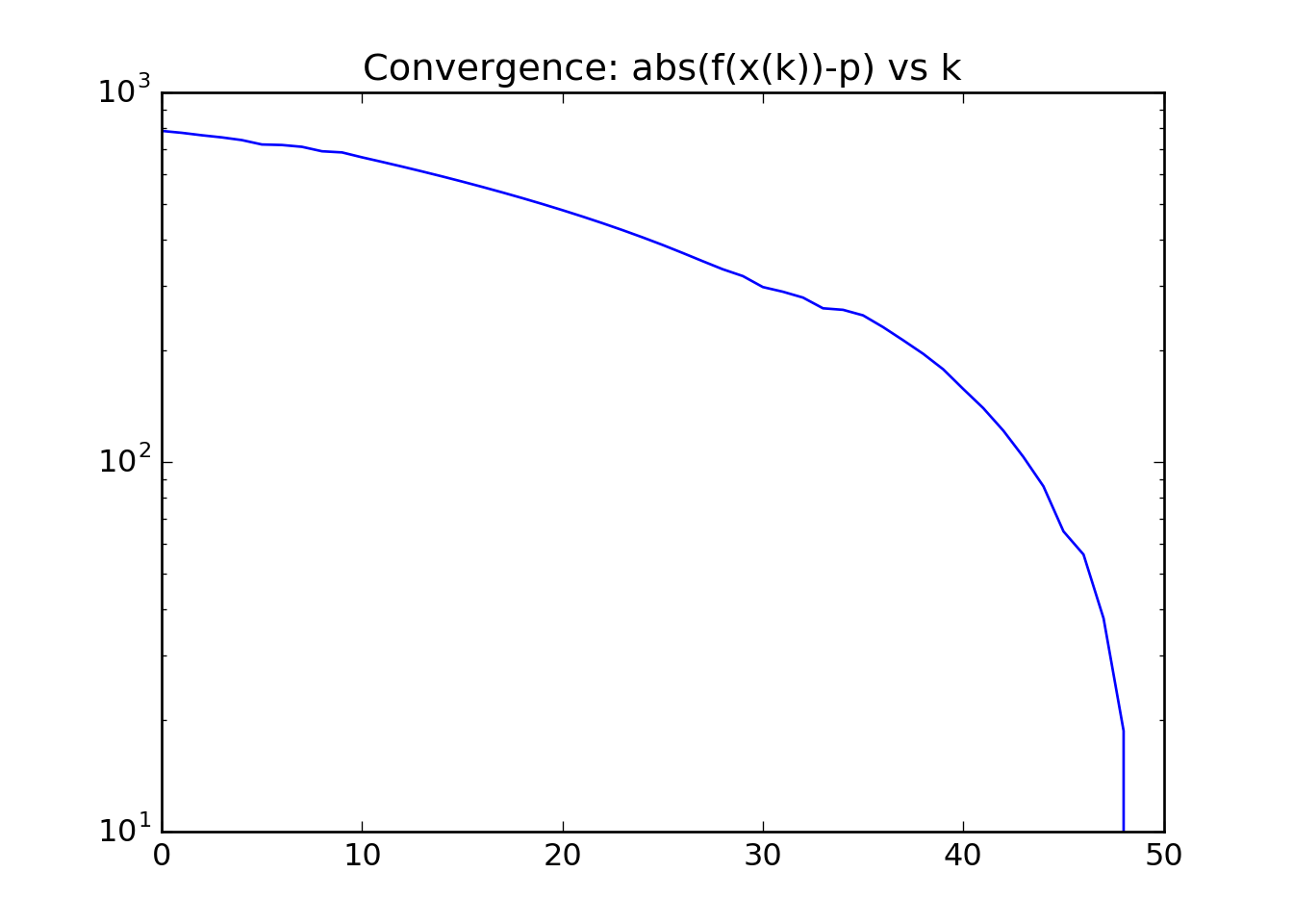
    fp = [abs(f-log.f[-1]) for f in log.f]
    plt.plot(log.k,fp)
    plt.yscale('log')
    plt.title('Convergence: abs(f(x(k))-p) vs k')
    #plt.xlim([0,27])
    plt.show()
    plt.clf()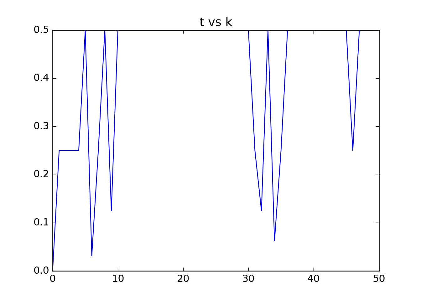

Analyzing our output

• We see that we indeed have quadratic convergence between the function at each step and our best guess of what the optimial value is; the \(f(x^{(\mathrm{kmax})})\).

Suggested Tutorials/References

• Convex Optimization Boyd and Vandenberg