Key questions we must address

• How do we recursively update \(x\) to approach \(x^*\)?
  • Answer: Standard descent methods use the following update term, \(x^{(k+1)}=x^{(k)}+t^{(k)}\Delta x^{(k)}\). While there is some freedom in our choice of \(t\) and \(\Delta x\), we must make sure that basic convex requirements hold; such as \(f(x^{(k+1)})<f(x^{(k)})\). What this means is that with each step we must be approaching a value of \(x\) that brings us closer to \(p^*\).
• How do we determine \(\Delta x_{nt}\)?
  • Answer: \(\Delta x_{nt}=-\frac{f'}{f''}\). This choice minimizes the second order taylor expansion of \(f(x+\Delta x_{nt})\), solves the linearized optimality condition for \(f'(x+\Delta x_{nt})\), and is the steepest descent direction at x in local Hessian norm.
• How do we determine \(t\)?
  • Answer: In our case we are considering the pure method so \(t=1\). However, we can use a line search method such as exact or back-tracking do solve for \(t\).
• How do we know when to stop?
  • Answer: We define the decrement as \(\lambda = \sqrt{\frac{f'(x)^2}{f''(x)}}\) and choose a stopping criterion of \(\frac{\lambda^2}{2}\le \epsilon\).

Psuedo code for Newton’s Method

• Given:
  • \(x_0\), \(x \in \mathrm{dom}(f)\)
  • \(\epsilon\), \(\epsilon>0\)
• Repeat:
  1. Compute \(\lambda\) and \(\Delta x_{nt}\)
  2. Quit if stopping criterion is reached
  3. Determine \(t\)
  4. Update \(x\)

Code for Newton’s Method

Now it’s time to code this thing up. Although I’m using python I will be trying to use basic structures that can be universally coded using any language.

#--------------------------------
#   Libraries
#--------------------------------
import sys
import numpy
import math
import matplotlib.pyplot as plt
#--------------------------------
#   Modules
#--------------------------------
def f(x):
  return math.log(2*math.cosh(x))

def d1_f(x):
  #---  d1_f(x) = f'(x)
  return math.tanh(x)

def d2_f(x):
  #---  d2_f(x) = f''(x)
  return (math.cosh(x)**(-1))**2

class Log:
  k=[]
  x=[]
  fp=[]#f(x)-p*
  def __init__(self,name):
    self.name = name
  def record(self,k,x,fp):
    self.k.append(k)  
    self.x.append(x)
    self.fp.append(fp)

def newton_method_pure(x0,p,kmax,e):
  #print 'Running newton_method() ...'
  log=Log('newton_method_pure')
  log.record(0,x0,f(x0)-p)
  k=1 #initialize step number
  x=x0 #initialize x
  t=1 #required for pure case
  while k<kmax:
    lamb = math.sqrt((d1_f(x)**2)/d2_f(x))
    if (lamb**2)/2 <= e:
      #print '... stopping criterion reached'
      break
    x_step = -(d1_f(x)/d2_f(x))
    x += t*x_step
    log.record(k,x,f(x)-p)
    k+=1
  return log
#--------------------------------
#   Main
#--------------------------------
if __name__ == "__main__":
    #---------------------------------
    #   Visualize functions    
    #---------------------------------
    x = [-2.+0.1*float(i) for i in range(0,40)]
    plt.plot(x,[f(y) for y in x])
    plt.plot(x,[d1_f(y) for y in x])
    plt.plot(x,[d2_f(y) for y in x])
    plt.title('functions for pure newton')
    plt.legend(['f(x)','d1_f(x)','d2_f(x)'])
    plt.show()
    plt.clf()
    #---------------------------------
    #   Run Solver
    #---------------------------------
    x0=1.0
    x_opt=0.0
    p=f(x_opt)
    kmax=10
    e=0.000001
    log=newton_method_pure(x0,p,kmax,e)
    plt.plot(log.k,log.fp)
    plt.yscale('log')
    plt.title('convergence: abs(f(x(k))-p) vs k')
    plt.show()
    plt.clf()

Analyzing our output

• The pure newtons method requires the step length be \(t=1\). We can determine \(t\) using exact or back-tracking methods by adding in a sub-step to our code.

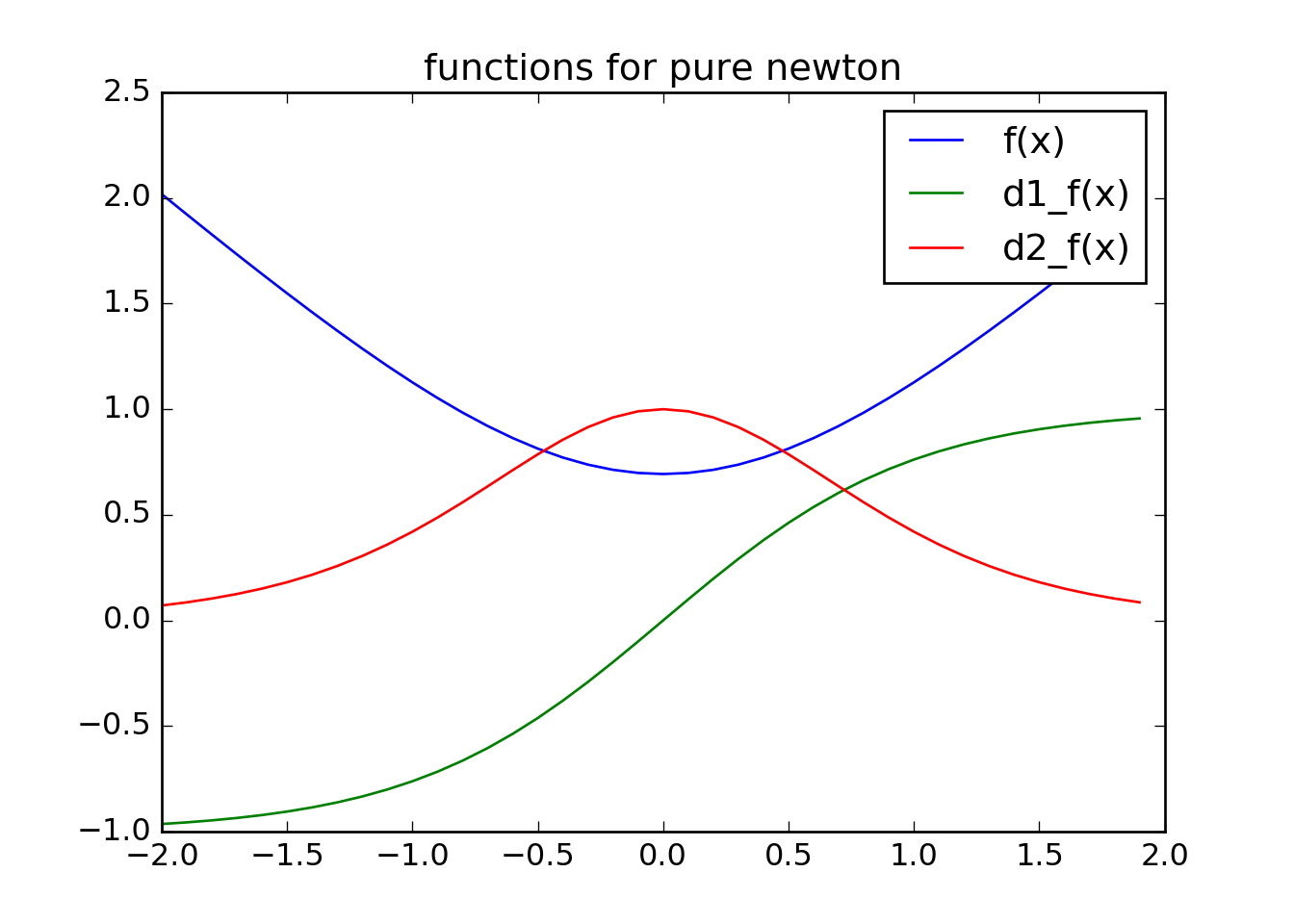
• Visually we see that \(f(x)\) is indeed convex. If not this solver will not work.

• In this case we can use our plots to identify what \(p^*\) and \(x^*\) are.

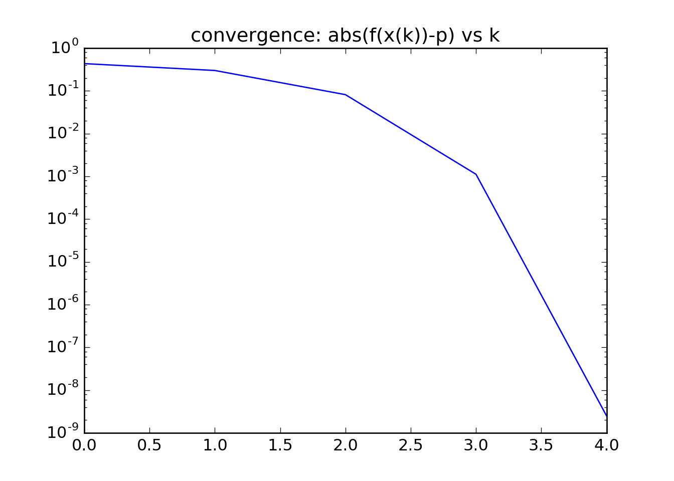
• We desire quadratic convergence between the function at each step and the optimal value.

• Quadratic convergence only occurs when we are close to the optimum solution. This is a major problem with Newtons method, and is illustrated by changing our initial point from 1.0 to 1.1. Try this out for yourself.

Changing things up

• Change modules for \(f(x)\), \(f'(x)\), and \(f''(x)\). This will require changes in \(x_0\) and \(p\).

Suggested Tutorials/References

• Convex Optimization Boyd and Vandenberg